Level
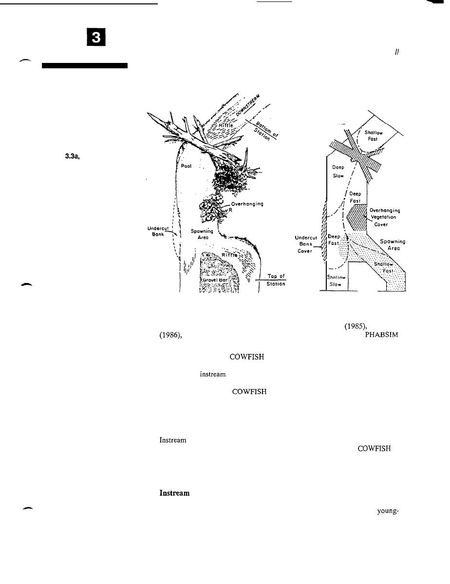
Figure
b Stream section
diagrams to illustrate detailed
mapping analyses of fish
habitat. (after Oswood and Barber
1982)
iparian
Vegetation
habitat model variables remain stable or show little fluctuation, then the model
assumes fish populations will also remain stable. Mathur et al.
Karr et al.
and Platts and Nelson (1988) have reviewed models based on
and have found limitations to their use.
The US Forest Service
model (Lloyd 1986) was designed for use in
the western United States for estimating past and current livestock impacts on
riparian and
conditions. The model is not intended to estimate fish
population variables or to replace current models developed for that purpose;
however, the results of
may be included in the Habitat Suitability
Index (Hickman and Raleigh 1982) to estimate optimum and existing catchable
fish populations. The geographic range for model development is Nevada, Utah,
Montana, and Idaho. The input variables include the extent of streambank
undercut, vegetation overhang, and bare soil or trampling.
variables include cobble embeddedness,
width, and depth. Stream
gradient and soil type are also considered. Shepard
(1989) used
to
evaluate livestock impacts in Montana and found
the model produced both
reasonable and imprecise estimates of catchable trout
depending upon the species
composition of the stream.
Habitat Parameters. Analysis of some life cycle and biotic interac-
tions may be necessary if impacts go beyond effects of pollutants and habitat.
Monitoring life cycle conditions needed for spawning, embryo survival,
of-the-year hiding, and the requirements for juveniles and adults may be useful,
with some evaluations focusing on the requirements for one or more life cycle
stages. Predator-prey relationships may also be assessed. Habitat requirements for
forage fishes may be a part of habitat analysis.
3.24


 Previous Page
